The Generic Mapping Tools (GMT)
A tutorial to make your own beautiful maps with GNU tools

The Generic Mapping Tools (GMT) are an open source collection of ~65 tools for manipulating geographic and Cartesian data sets (including filtering, trend fitting, gridding, projecting, etc.) and producing Encapsulated PostScript File (EPS) illustrations ranging from simple x-y plots via contour maps to artificially illuminated surfaces and 3-D perspective views; the GMT supplements add another ~70 more specialized tools. GMT supports over 30 map projections and transformations and comes with support data such as GSHHS coastlines, rivers, and political boundaries.
GMT allows both highly qualified professionals and newbies to make wonderful maps of any region of the world. However, GMT is far from being user friendly and it uses so much computer resources (RAM memory). It is my aim in this tutorial to explain how to make maps, and where to get further information to fill them up with all kinds of useful information. Using Debian (right now 7.x Wheezy) it is very easy to install GMT and to get it up and running. So let's get started.
In Debian Wheezy we may install the version v4.5.7, which is not the latest, but as usual, it works just fine:
sudo apt-get install gmt gmt-gshhs-full csh awk
The packages csh and awk provides us with tools to run scripts and edit files.
A last step is necessary. The variable PATH does not contain gmt's binaries path (/usr/lib/gmt/bin). Edit the file ~/.bashrc, and add the following at the end of the file:
# setting path for the gmt program
PATH="$PATH:/usr/lib/gmt/bin"
To make sure the system reads the configuration files it is good to logout and login again (or reboot). After that open a terminal and type:
echo $PATH
to check if everything is fine. First step accomplished!
 In our first map, we shall draw a beautiful physical map.
GMT provides data about the coastlines only, but it is ready to read data, as for instance Digital Elevation Maps (DEM), to plot detailed physical maps.
There are several sources of free DEMs.
To begin, we shall use data from the Geographic Information Network of Alaska (GINA), so thank you so much to provide such valuable data.
GINA's DEMs Results are provided as eight GMT grid files covering a -180° to +180° longitude and -90° to 90° latitude.
To facilitate ease of use without loss of resolution, all data have been sampled and merged into identically registered 30-s grids.
The actual resolutions of the topography and bathymetry data are roughly 30 arc s (0.66 km at 45° latitude) and 2 arc min (2.6 km at 45° latitude), respectively.
We download the bzipped data from here.
Be ready to download heavy files, so it may take a while to get everything you need.
If you are only interested in a certain region of the world, you should download only the files containing data of that region.
After downloading, you uncompress the data and put everything in the same folder, for instance ~/Documents/gina.
In our first map, we shall draw a beautiful physical map.
GMT provides data about the coastlines only, but it is ready to read data, as for instance Digital Elevation Maps (DEM), to plot detailed physical maps.
There are several sources of free DEMs.
To begin, we shall use data from the Geographic Information Network of Alaska (GINA), so thank you so much to provide such valuable data.
GINA's DEMs Results are provided as eight GMT grid files covering a -180° to +180° longitude and -90° to 90° latitude.
To facilitate ease of use without loss of resolution, all data have been sampled and merged into identically registered 30-s grids.
The actual resolutions of the topography and bathymetry data are roughly 30 arc s (0.66 km at 45° latitude) and 2 arc min (2.6 km at 45° latitude), respectively.
We download the bzipped data from here.
Be ready to download heavy files, so it may take a while to get everything you need.
If you are only interested in a certain region of the world, you should download only the files containing data of that region.
After downloading, you uncompress the data and put everything in the same folder, for instance ~/Documents/gina.
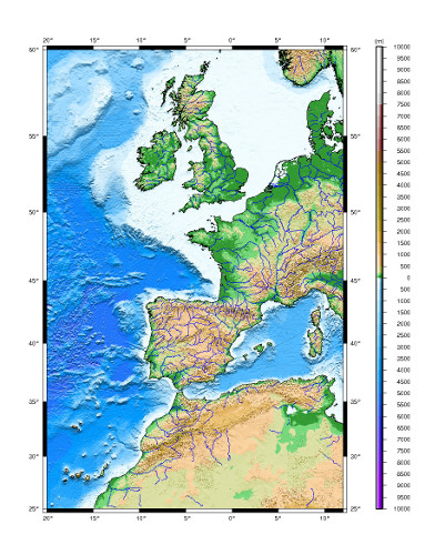
To draw the map we shall run a script which contains all the necessary instructions, that we shall explain in a certain detail from now on. We will make a map of a region of western europe. The content of the script follows. It is quite commented so you can alter it depending on what you need.
#!/bin/csh
# Name of the file containing the map in eps format
set PSFILE = iberica.eps
# Name of the file containing GINA's grid file used to make the map
set GRD = iberica2.grd
# Parameters Setting
# gmtdefaults lists the GMT parameter defaults if the option -D is used.
# We write system defaults to the file .gmtdefaults
# After running this script you also find .gmtdefaults4 file containing the parameters used in our maps
gmtdefaults -D >! .gmtdefaults
# MEASURE_UNIT: Sets the unit length. Choose between cm, inch, m, and point. [cm].
# Note that, in GMT, one point is defined as 1/72 inch or 0.35278 mm (the PostScript definition).
gmtset MEASURE_UNIT point
# PAPER_MEDIA: Paper used (list with type, width and height in points)
# A3 842 1190
# A4 595 842
# A5 421 595
# To indicate you are making an EPS file, append '+' to the media name.
# Then, GMT will attempt to issue a tight bounding box [Default Bounding Box is the paper dimension].
# The '+' option does not work properly in my case, please be carefull. # gmtset PAPER_MEDIA a4+
gmtset PAPER_MEDIA Custom_675x842
# ANOT_FONT_SIZE: controls the size of the characters/numbers in psscale (to make scale bars)
# and in some other other tools.
gmtset ANOT_FONT_SIZE 9p
# LABEL_FONT_SIZE: Font size (> 0) for labels (e.g. Axis labels with coordinates)
gmtset LABEL_FONT_SIZE 10p
# DEGREE_SYMBOL: Choose between ring, degree, colon, or none [ring]
gmtset DEGREE_SYMBOL degree
# gmtset PLOT_DEGREE_FORMAT
# The template is in general of the form [+|-]D or [+|-]ddd[:mm[:ss]][.xxx][F].
# By default, longitudes will be reported in the -180/+180 range.
# The various terms have the following purpose:
# + -----> Output longitude in the 0 to 360 range [-180/+180]
# - -----> Output longitude in the -360 to 0 range [-180/+180]
# D -----> Use D_FORMAT for floating point degrees.
# ddd ---> Fixed format integer degrees
# : -----> delimiter used
# mm ----> Fixed format integer arc minutes
# ss ----> Fixed format integer arc seconds
gmtset PLOT_DEGREE_FORMAT D
# PAGE_ORIENTATION: Choose portrait or landscape [landscape].
# gmtset PAGE_ORIENTATION landscape
# You may check more parameters here: http://gmt.soest.hawaii.edu/gmt/html/man/gmtdefaults.html
# Creation of color palette to make the map
#
# makecpt is a utility that will help you make color palette tables (cpt files).
# You define an equidistant set of contour intervals
# and create a new cpt file based on an existing master cpt file.
# The resulting cpt file can be reversed relative to the master cpt,
# and can be made continuous or discrete.
# The color palette includes three additional colors beyond the range of z-values.
# These are the background color (B) assigned to values lower than the lowest z-value,
# the foreground color (F) assigned to values higher than the highest z-value,
# and the NaN color (N) painted whereever values are undefined.
# If the master cpt file includes B, F, and N entries, these will be copied into the new master file.
# If not, the parameters COLOR_BACKGROUND, COLOR_FOREGROUND, and COLOR_NAN from
# the .gmtdefaults4 file or the command line will be used.
#
# The option -C selects the master color table to use in the interpolation.
# Choose among the built-in tables (type makecpt to see the list) or
# give the name of an existing cpt file [Default gives a rainbow cpt file].
# The following line created the palette tmp.cpt. It is good you check this file with a text editor.
makecpt -Cglobe >! tmp.cpt
# Creation of the grid file to make the map
#
# grdcut will produce a new output_file.grd file which is a subregion of input_file.grd.
# The subregion is specified with -R the specified range must not exceed the range of input_file.grd.
# If in doubt, run grdinfo to check range.
# Complementary to grdcut there is grdpaste, which will join together two grid files along a common edge.
#
# We need the following two regions for our map of western europe based in GINA. Please change for other regions:
# You only need to run the following command only ONCE!
grdpaste North_West.grd North_East.grd -Giberica.grd
# Then we extract a region of coordinates
# min. longitude = 20 degrees; max longitude = 12 degrees;
# min. latitude = 25 degrees; max latitude = 60 degrees;
grdcut iberica.grd -Giberica2.grd -R-20/12/25/60
# To make the map more beautiful and informative, we will add a light and compute some shadows,
# so mountain's shape become much more apparent.
#
# grdgradient: Compute directional derivative or gradient from 2-D grid file representing z(x,y).
#-Aazim Azimuthal direction for a directional derivative;
# azim is the angle in the x,y plane measured in degrees positive clockwise from north (the +y direction) toward east (the +x direction).
#-A0 means illumination from north.
#-N -Ne normalizes using a cumulative Laplace distribution. -Nt normalizes using a cumulative Cauchy distribution
#-M use this option to make sure the output has good units.
#-G Name of the output grid file for the directional derivative.
# The first parameter is the input file, which is obtained from $GRD (see the definition of GRD at the beginning of the script)
grdgradient $GRD -Giberica2.int -A0 -Nt -M
# grdimage makes the map using the grid file and the palette file that we already created.
#
# grdimage: Create grayshaded or colored image from a 2-D netCDF grid file
# -J Selects the map projection.
# For a cylindrical projection we may have -JMscale, where scale is along parallel (1:xxxx or UNIT/degree).
# -B Sets map boundary annotation and tickmark intervals;
# -P Selects portrait plotting mode.
# -K More PostScript code will be appended later
grdimage $GRD -R-20/12/25/60 -Iiberica2.int -JM450 -B5 -Ctmp.cpt -P -K >! $PSFILE
# pscoast: To plot land-masses, water-masses, coastlines, borders, and rivers.
#
# -D Selects the resolution of the data set to use ((f)ull, (h)igh, (i)ntermediate, (l)ow, and (c)rude).
# -I Draw rivers. Specify the type of rivers and [optionally] append pen attributes
# Types of rivers:
# 1 = Permanent major rivers, 2 = Additional major rivers, 3 = Additional rivers, 4 = Minor rivers,
# 5 = Intermittent rivers - major, 6 = Intermittent rivers - additional, 7 = Intermittent rivers - minor
# 8 = Major canals, 9 = Minor canals, 10 = Irrigation canals
# a = All rivers and canals (1-10), r = All permanent rivers (1-4), i = All intermittent rivers (5-7)
# c = All canals (8-10)
# For pen attributes you should indicate [pen width in points]/R/G/B
# -W Draw shorelines [Default is no shorelines]. Append pen attributes [Defaults: width = 0.25p, color = black, texture = solid]
# -O Selects Overlay plot mode [Default initializes a new plot system].
pscoast -R-20/12/25/60 -JM450 -Df -Ia/0.05p/0/0/254 -W1/0 -O -K>> $PSFILE
# psscale plots scales on maps.
# Variations in intensity due to shading/illumination may be displayed by setting the option âI.
# Colors may be spaced according to a linear scale, all be equal size, or by providing a file with individual tile widths.
# -D Defines the position of the center/top (for horizontal scale) or center/left (for vertical scale) and the dimensions of the scale.
# Give a negative length to reverse the scalebar. Append h to get a horizontal scale [Default is vertical].
# -B Set annotation, tick, and gridline interval for the colorbar.
psscale -D500/350/700/10 -Ctmp.cpt -I -Ba500f500/a500f500:"(m)": -O >> $PSFILE
You can try this script by copying everything to a file, for instance script.csh. Make the file executable:
sudo chmod +x script.csh
and then you execute it. You will get a map identical to the one you can see in the picture.
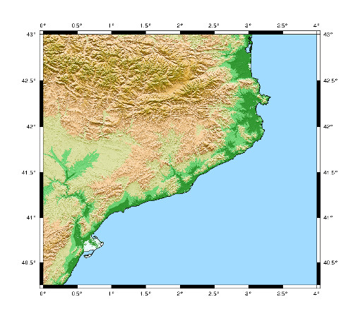
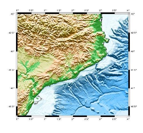
GINA's data is good to plot maps of a continent or a piece of a continent. To map a smaller region with higher detail, it is better to use SRTM data as we do in the next section. We will make a map of a region corresponding to Catalunya (north-east Spain).
3. Using high resolution data from SRTM to make maps of small regions
 SRTM stands for Shuttle Radar Topography Mission; is a digital elevation model that is derived from radar interferometry data obtained during a space shuttle mission.
The dataset covers most of the globe, except polar regions, i.e. between 56° S and 60° N, in a resolution of 3 arc seconds (approx. 90m resolution over 80% of the globe).
This data is currently distributed free of charge by USGS and is available for download from the National Map Seamless Data Distribution System, or the USGS ftp site.
SRTM stands for Shuttle Radar Topography Mission; is a digital elevation model that is derived from radar interferometry data obtained during a space shuttle mission.
The dataset covers most of the globe, except polar regions, i.e. between 56° S and 60° N, in a resolution of 3 arc seconds (approx. 90m resolution over 80% of the globe).
This data is currently distributed free of charge by USGS and is available for download from the National Map Seamless Data Distribution System, or the USGS ftp site.
This data is provided in an effort to promote the use of geospatial science and applications for sustainable development and resource conservation in the developing world. Digital elevation models (DEM) for the entire globe, covering all of the countries of the world, are available for download. The SRTM 90m DEM's have a resolution of 90m at the equator, and are provided in mosaiced 5 deg x 5 deg tiles for easy download and use. All are produced from a seamless dataset to allow easy mosaicing. These are available in both ArcInfo ASCII and GeoTiff format. We are interested in the ArcInfo ASCII format because we know how to change this format to another format that can be accepted by the GMT routines. So the first step is to get into the web page (just click in the link above) and download the files corresponding to the region you are interested in.
If the data is downloaded in the ArcInfo ASCII format, it can be converted to the usual xyz format (lon, lat, elevation) using the following script: esri-asc2xyz.pl
./esri-asc2xyz.pl < srtm_37_04.asc > srtm_37_04.xyz
The xyz file may then be converted to GMT grd using the GMT program xyz2grd:
xyz2grd srtm_37_04.xyz -R0/5/40/45 -Gsrtm_37_04.grd -I3c
The region, given in the -R parameter, can be determined using GMT's minmax tool:
minmax srtm_37_04.xyz
or reading the information of each tile you downloaded. minmax provides an information that looks like:
srtm_37_04.xyz: N = 36012001 <-0.000416618268153/4.99958338173> <39.9995835754/44.9995835754> <-9999/3383>
The last data couple corresponds to the maximum and minimum height (z coordinate) in the file. The oceans and seas correspon to a value of -9999. To make a nice map we may interested to change this value to another, for instance -1250 so we get a nice blue color for the sea regions. To do that we use grdclip:
grdclip srtm_37_04.grd -Gsrtm_37_04_clip.grd -Sb-9000/-1250 -V0/5/40/45
The -Sb-9000/-1250 option means that any value lower than -9000 becomes -1250.
You can use now the file srtm_37_04_clip.grd to make a map in the same way we used data from GINA in the last section:
#!/bin/csh
# Name of the file containing the map in eps format
set PSFILE = cat.eps
# Name of the file containing SRTM's grid file used to make the map
set GRD = srtm_37_04_clip.grd
gmtdefaults -D >! .gmtdefaults
gmtset MEASURE_UNIT point
gmtset PAPER_MEDIA Custom_580x540
gmtset ANOT_FONT_SIZE 9p
gmtset LABEL_FONT_SIZE 10p
gmtset DEGREE_SYMBOL degree
gmtset PLOT_DEGREE_FORMAT D
makecpt -Cglobe >! tmp.cpt
grdgradient $GRD -Giberica2.int -A0 -Nt -M
grdimage $GRD -R0/4/40.25/43 -Iiberica2.int -JM450 -B0.5 -Ctmp.cpt -P -K >! $PSFILE
pscoast -R-0/4/40.25/43 -JM450 -Df -W1/0 -O >> $PSFILE
This script will make a map like the one in the picture.
If you plot a map corresponding to several tiles it is convenient to combine them. Actually pairs of adjacent tiles can be combined. This is useful e.g. for an illumination map created using grdgradient, as we did in the last section, where all grid tiles should be normalized in the same way:
grdpaste grid1.grd grid2.grd -Gcombined.grd
Using grdpaste multiple times you can get a single file for a wide area.
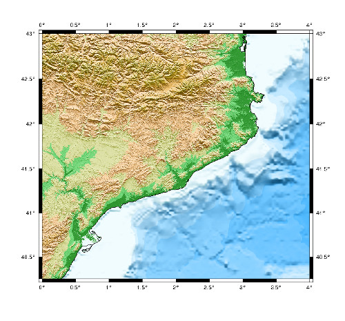 Imagine now that we wish to use GINA data only for the ocean
and SRTM data only for land. To combine both data sets we do the following:
Imagine now that we wish to use GINA data only for the ocean
and SRTM data only for land. To combine both data sets we do the following:
#!/bin/csh
# We start preparing a file from GINA data
# Clip GINA data so only ocean data remains
# The option -Sa sets all data higher than a certain number (-10.0m) to a certain value (-10.0m)
# -G indicates output file
grdclip cat_gina.grd -Gcat_gina2.grd -Sa-10.0/-10.0 -V
# Resample GINA data to the same resolution of SRTM data
# This is necesseray to combine both data sets
# The option -F forces pixel node registration on output grid.
# [Default is same registration as input grid].
grdsample cat_gina2.grd -I3c -Gcat_gina3.grd -R0/5/40/45 -F
# The file cat_gina3.grd is now ready for our purpose
# We now prepare a file from srtm data
#Clip SRTM data so "ocean data" becomes NaN
grdclip cat_srtm.grd -Gcat_srtm_clip.grd -Sb-1000/NaN -V
#Resample SRTM data so both data sets have data on the same points (nodes)
grdsample cat_srtm_clip.grd -I3c -Gcat_srtm_clip2.grd -R0/5/40/45 -F -Qn
#Combine both data sets, so NaN data from SRTM becomes data from GINA
#-N Turns off strict domain match checking when multiple grids are manipulated
# [Default will insist that each grid domain is within 1e-4 * grid_spacing of the domain of the first grid listed].
# The operator AND returns NaN if A and B == NaN, B if A == NaN, else A.
grdmath -N cat_srtm_clip2.grd cat_gina3.grd AND = srtm_gina.grd
# The file srtm_gina.grd is the final grid file to make the map
 The final file srtm_gina.grd can be used to make the map we wished (the one in the picture) using the same script as before (the one in the last section).
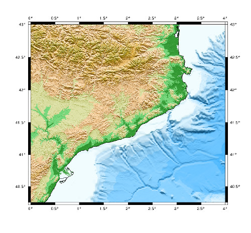
Instead of using bathymetry data from GINA, you can get it from ETOPO1. ETOPO1 contains both land topography and ocean bathymetry with a resolution of 1 minute of arc for any region of the world. It was built from numerous global and regional data sets, and is available in "Ice Surface" (top of Antarctic and Greenland ice sheets) and "Bedrock" (base of the ice sheets) versions. If you are interested in mapping a wide area you may also download ETOPO1 at a global scale. You can get netCDF grid files from NOAA and use them directly in our GMT scripts. ETOPO1 data set is very suitable to plot World Maps, since 1 minute of arc resolution is more than enough for this purpose.
After you get the desired ETOPO1 data, you can use the same script to transform data in such way that it can be merged with SRTM data. The resulting map looks a bit better than GINA's one (watch the second map in this section).

![]() There are so many different formats in which people provide their data. It is a wonderful proof of human stupidity at its best.
Anyway, to get further we need a program to transform data so we can use it with GMT. A very nice open source program that will allow us to perform such transformation is SAGA GIS.
It was originally developed by a small team at the Department of Physical Geography, University of Göttingen, Germany,
and is now being maintained and extended by an international developer community.
There are so many different formats in which people provide their data. It is a wonderful proof of human stupidity at its best.
Anyway, to get further we need a program to transform data so we can use it with GMT. A very nice open source program that will allow us to perform such transformation is SAGA GIS.
It was originally developed by a small team at the Department of Physical Geography, University of Göttingen, Germany,
and is now being maintained and extended by an international developer community.
SAGA is the abbreviation for System for Automated Geoscientific Analyses and it's a Geographic Information System (GIS) software. SAGA has been designed for an easy and effective implementation of spatial algorithms and it offers a comprehensive, growing set of geoscientific methods. It provides an easily approachable user interface with many visualisation options. It runs under Windows and Linux operating systems and it is a Free Open Source Software (FOSS). You can get some important documents (tutorials, manuals, etc) here.
SAGA is available from Debian repositories for Debian Squeeze and Jessie, but not for the current stable version, Wheezy. If you are using Debian Wheezy a good option is to compile the program. It is necessary to install a few libraries from the repositories. Make sure you install the libraries and the corresponding headers and development files for the following list:
- wxWidgets 3.0.0
- GDAL 1.8.0
- Proj4
- Haru Free PDF Library (optional)
- libLAS 1.2 (optional)
- opencv (optional)
- vigra (optional)
Then you download the source code from sourceforge. To compile and install it just follow the standart procedure and run:
./configure
make
sudo make install
Of course you check any errors in the process. I was lucky enough to get into a long and smooth compilation process. After installing the program you are ready for the next challenge.
 In the first section we draw a map with rivers.
However, if try to use GMT's rivers for a small region, then we realize we need a more accurate data base.
HydroSHEDS (Hydrological data and maps based on SHuttle Elevation Derivatives at multiple Scales) provides hydrographic information for
regional and global-scale applications. HydroSHEDS offers a suite of geo-referenced data sets (vector and raster), including stream networks, watershed boundaries,
drainage directions, and ancillary data layers such as flow accumulations, distances, and river topology information.
In the first section we draw a map with rivers.
However, if try to use GMT's rivers for a small region, then we realize we need a more accurate data base.
HydroSHEDS (Hydrological data and maps based on SHuttle Elevation Derivatives at multiple Scales) provides hydrographic information for
regional and global-scale applications. HydroSHEDS offers a suite of geo-referenced data sets (vector and raster), including stream networks, watershed boundaries,
drainage directions, and ancillary data layers such as flow accumulations, distances, and river topology information.
HydroSHEDS is derived from elevation data of the Shuttle Radar Topography Mission (SRTM) at 3 arc-second resolution. The original SRTM data have been hydrologically conditioned using a sequence of automated procedures. Manual corrections were made where necessary. Preliminary quality assessments indicate that the accuracy of HydroSHEDS significantly exceeds that of existing global watershed and river maps. The goal of developing HydroSHEDS was to generate key data layers to support regional and global analyses resolution and extent that had previously been unachievable. Available resolutions range from 3 arc-second (approx. 90 meters at the equator) to 5 minute (approx. 10 km at the equator) with seamless near-global extent.
The available data for river streams corresponds to a resolution of 15 arc-second (approx. 500 m at the equator ). The data called "RIVER NETWORK" is the one we need and we may freely download it from here. The data has a Vector data format called "ESRI Shapefile" format. The vector data sets distributed with HydroSHEDS, i.e. river lines (RIV) and basin polygons (BAS), are being made available in ESRI Shapefile format (ESRI 1998). A HydroSHEDS shapefile typically consists of five main files (.dbf, .sbn, .sbx, .shp, .shx). Additionally, basic metadata information is provided both in XML format (.xml) and in HTML format (.htm) following the FGDC standard. Projection information is provided in an ASCII text file (.prj). All shapefiles are in geographic (latitude/longitude) projection, referenced to datum WGS84.
 You download the data you need and then the game starts (first thing you unpack it).
We shall use the files with .shp extension which contain the information of river streams.
GMT does not recognize the ESRI shape file format, so we use SAGA GIS to read those files and transform them into something GMT may read (.xyz text file).
We work now over european rivers (follow the same explanation with your favorite area) Start SAGA and import the data going to File -> Shapes -> Load and select the file eu_riv_15s.shp.
Takes a second or so to load.
To check the data you can make a map immediatly by just going to the "Manager" window, data tab, right click over the name of the file and select "Add to map".
An awful solid red map appears... zoom it to see the rivers! You will see that almost every water stream should be there! Incredible!
You download the data you need and then the game starts (first thing you unpack it).
We shall use the files with .shp extension which contain the information of river streams.
GMT does not recognize the ESRI shape file format, so we use SAGA GIS to read those files and transform them into something GMT may read (.xyz text file).
We work now over european rivers (follow the same explanation with your favorite area) Start SAGA and import the data going to File -> Shapes -> Load and select the file eu_riv_15s.shp.
Takes a second or so to load.
To check the data you can make a map immediatly by just going to the "Manager" window, data tab, right click over the name of the file and select "Add to map".
An awful solid red map appears... zoom it to see the rivers! You will see that almost every water stream should be there! Incredible!
To export de data into a .xyz file go to the window "Manager", select the "tools" tab -> Import/Export Shapes -> Export Shapes to XYZ. In the "properties" window a menu just appears. Now in "Shapes" you select the file already opened, in Attribute you select UP_CELLS. Attribute corresponds to Z coordinates and UP_CELLS will be a number measuring the importance of the water flow. Do not save table header, select "*" as "Separate Line/Polygons forms" and finally select the name of the output file (with its full path!). Click on execute and you get your new .xyz file!
The Z coordinate corresponds to the amount of upstream area (in number of cells) draining into each cell. A drainage direction layer is used to define which cells flow into the target cell. The number of accumulated cells is essentially a measure of the upstream catchment area. However, since the cell size of the HydroSHEDS data set depends on latitude, the cell accumulation value cannot directly be translated into drainage areas in square kilometers. Only rivers with upstream drainage areas exceeding a certain threshold are selected: for the 15 arc-second resolution a threshold of 100 upstream cells has been used. The vectorized river reaches are currently attributed with the maximum flow accumulation (in number of cells) occurring within each river reach.
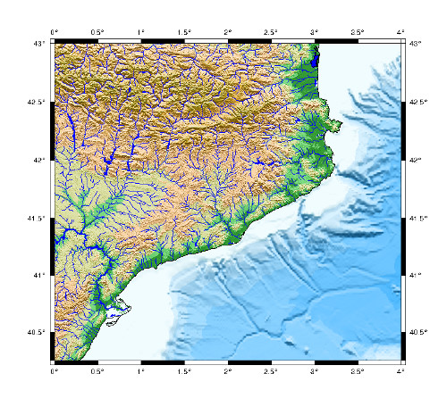
When doing the map, we shall take into account the value of Z to determine the width of the lines representing the rivers. A logarithmic scale may be appropiate. We called the river file rius.xyz. To plot the rivers we add the following to the script (for instance before the pscoast function):
# Plots river streams
awk '{ if($2 == "") { print "*" } else if ($3 <= 1000) {printf("%f %f %f\n", $1, $2, $3)} }' rius.xyz | \
psxy -R -JM -M -W0.5/0/0/255:td -O -K >> $PSFILE
awk '{ if($2 == "") { print "*" } else if ($3 > 1000 && $3 <= 5000) {printf("%f %f %f\n", $1, $2, $3)} }' rius.xyz | \
psxy -R -JM -M -W1/0/0/255:td -O -K >> $PSFILE
awk '{ if($2 == "") { print "*" } else if ($3 > 5000 && $3 <= 25000) {printf("%f %f %f\n", $1, $2, $3)} }' rius.xyz | \
psxy -R -JM -M -W2/0/0/255:td -O -K >> $PSFILE
awk '{ if($2 == "") { print "*" } else if ($3 > 25000 && $3 <= 125000) {printf("%f %f %f\n", $1, $2, $3)} }' rius.xyz | \
psxy -R -JM -M -W3/0/0/255:td -O -K >> $PSFILE
awk '{ if($2 == "") { print "*" } else if ($3 > 125000 && $3 <= 625000) {printf("%f %f %f\n", $1, $2, $3)} }' rius.xyz | \
psxy -R -JM -M -W4/0/0/255:td -O -K >> $PSFILE
awk '{ if($2 == "") { print "*" } else if ($3 > 625000 && $3 <= 15625000) {printf("%f %f %f\n", $1, $2, $3)} }' rius.xyz | \
psxy -R -JM -M -W5/0/0/255:td -O -K >> $PSFILE
awk '{ if($2 == "") { print "*" } else if ($3 > 15625000 && $3 <= 78125000) {printf("%f %f %f\n", $1, $2, $3)} }' rius.xyz | \
psxy -R -JM -M -W6/0/0/255:td -O -K >> $PSFILE
awk '{ if($2 == "") { print "*" } else if ($3 >78125000) {printf("%f %f %f\n", $1, $2, $3)} }' rius.xyz | \
psxy -R -JM -M -W7/0/0/255:td -O -K >> $PSFILE
If you are not familiar with awk, notice that "$1" represents the values of the first column, "$2" the values of the second column and so on. The awk instruction will read the file rius.xyz line per line and sends the output (produced by the function printf) to the function psxy of GMT. The option -W indicates the width and color of the line. The final result can be seen in the picture.
 A new 30-arc second resolution global topography/bathymetry grid
(SRTM30_PLUS)
has been developed from a wide variety of data sources.
Land and ice topography comes from the SRTM30 and ICESat topography, respectively.
Ocean bathymetry is based on a new satellite-gravity model where the gravity-to-topography ratio is calibrated using 298 million edited soundings.
A new 30-arc second resolution global topography/bathymetry grid
(SRTM30_PLUS)
has been developed from a wide variety of data sources.
Land and ice topography comes from the SRTM30 and ICESat topography, respectively.
Ocean bathymetry is based on a new satellite-gravity model where the gravity-to-topography ratio is calibrated using 298 million edited soundings.
This SRTM30_PLUS data consists of 33 files of global topography in the same format as the SRTM30 products distributed by the USGS EROS data center. The grid resolution is 30 second which is roughly one kilometer. In addition the global data are also available in a single large file ready for GMT!.
Land data are based on the 1-km averages of topography derived from the USGS SRTM30 grided DEM data product created with data from the NASA Shuttle Radar Topography Mission. GTOPO30 data are used for high latitudes where SRTM data are not available. Ocean data are based on the Smith and Sandwell global 1-minute grid between latitudes +/- 81 degrees. Higher resolution grids have been added from the LDEO Ridge Multibeam Synthesis Project, the JAMSTEC Data Site for Research Cruises, and the NGDC Coastal Relief Model. Arctic bathymetry is from the International Bathymetric Chart of the Oceans (IBCAO) [Jakobsson et al., 2003]. The data are also merged into a single large (1.9 Gbyte, 2-byte integer) file as well as smaller 1-minute and 2-minute netcdf versions.
In the regions I considered so far SRTM30_PLUS offers more detail than GINA or ETOPO1, which offer 1 minute of arc resolution at the most. Of course SRTM is still offering the highest resolution: 3 seconds of arc.
GLOBE is a 30-arc-second (1-km) gridded, quality-controlled global Digital Elevation Model (DEM). The final data is not as good as SRTM30_PLUS (see section 7), and data format is not easy to manage for GMT users. I do not recommend to use GLOBE, but if you are still interested, I explain now how to get GLOBE data into GMT.
First you download data (divided in 16 tiles) here. You can choose the option "all tiles in one .tgz" file. Then you put all the tiles in one single folder and run the following bash script:
#!/bin/bash
# Convert the original GLOBE files to the GMT *.grd format
FILES=(*10g)
LAT_S=(50 0 -50 -90)
LAT_N=(90 50 0 -50)
# Get the grid files from GLOBE original data
echo MAKING GRID FILES
for((y=0; y<=3; y++)); do
for(( x=0; x<=3; x++)); do
REGION="$((-180+$x*90))/$((-90+$x*90))/${LAT_S[$y]}/${LAT_N[$y]}"
xyz2grd ${FILES[$(($y*4+$x))]} -G${FILES[$(($y*4+$x))]}.grd -R$REGION -I30c -N-9999 -V -F -ZTLh
done
done
# MAKING global xyz file:
echo GLOBE.xyz
grd2xyz *.grd > GLOBE.xyz
# Conversion to GMT grd
echo GMT grd
xyz2grd GLOBE.xyz -Rd -F -GGLOBE.grd -I30c
This bash script is a modified (simplified, corrected and optimized) version of the one in this page. The final file GLOBE.grd may be used in the GMT routines.
 Drawing upon a variety of existing maps, data and information, WWF (worldwildlife) and the Center for Environmental Systems Research,
University of Kassel, Germany created the Global Lakes and Wetlands Database (GLWD).
The combination of best available sources for lakes and wetlands on a global scale (1:1 to 1:3 million resolution),
and the application of GIS functionality enabled the generation of a database which focuses in three coordinated levels on (1) large lakes and reservoirs,
(2) smaller water bodies, and (3) wetlands.
Drawing upon a variety of existing maps, data and information, WWF (worldwildlife) and the Center for Environmental Systems Research,
University of Kassel, Germany created the Global Lakes and Wetlands Database (GLWD).
The combination of best available sources for lakes and wetlands on a global scale (1:1 to 1:3 million resolution),
and the application of GIS functionality enabled the generation of a database which focuses in three coordinated levels on (1) large lakes and reservoirs,
(2) smaller water bodies, and (3) wetlands.
- Level 1 (GLWD-1) comprises the 3067 largest lakes (area >= 50 km2) and 654 largest reservoirs (storage capacity >=0.5 km3) worldwide, and includes extensive attribute data.
- Level 2 (GLWD-2) comprises permanent open water bodies with a surface area >= 0.1 km2 excluding the water bodies contained in GLWD-1. The approximately 250,000 polygons of GLWD-2 are attributed as lakes, reservoirs and rivers.
- Level 3 (GLWD-3) comprises lakes, reservoirs, rivers and different wetland types in the form of a global raster map at 30-second resolution. For GLWD-3, the polygons of GLWD-1 and GLWD-2 were combined with additional information on the maximum extents and types of wetlands. Class "lake" in both GLWD-2 and GLWD-3 also includes man-made reservoirs, as only the largest reservoirs have been distinguished from natural lakes.
We shall focus on Level 1 and Level 2 data, which contains lakes and reservoirs with a surface area >= 0.1 km2. The data in ESRI shapefiles format can be easily transformed into xyz files following the same procedures described in section 6. To plot the lakes we can use the psxy function as follows.
# Plots Lakes
awk '{ if($2 == "") { print "*" } else if ($3 > 0) {printf("%f %f %f\n", $1, $2-0.007, $3)} }' lakes.xyz | \
psxy -R -JM -M -L -W1/0/0/255:td -G0/0/255 -O -K >> $PSFILE
Notice the correction of 0.007 degrees in the latitude, which is necessary to make both data sets consistent. This is a correction of about 25 arc seconds. Level 3 data is provided within a resolution of 30 arc sec, so it seems consistent with the data accuracy. In the picture you can see all together, srtm for topography, etopo1 for bathymetry, Hydrosheds for rivers and GLWD for lakes for Catalunya (a region of northeast Spain).
We started working with SRTM data in section 3, 4 and 7. Resampled SRTM data to 250m resolutions (7.5 arc-s) for the entire globe are available https://hc.box.net/shared/1yidaheouv (Password: ThanksCSI!).
The data are in ARC GRID, ARC ASCII and Geotiff format, in decimal degrees and datum WGS84. They are derived from the USGS/NASA SRTM data. CIAT have processed this data to provide seamless continuous topography surfaces. Areas with regions of no data in the original SRTM data have been filled using interpolation methods described by Reuter et al. (2007). For ASCII format files the projection definition is included in .prj files.
The ARC ASCII format is very convenient for us because it is easy to get it into GMT. This time we use the function xyz2grd for that purpose:
xyz2grd -E srtm_w_250m.asc -Gsrtm_w_250m.grd
xyz2grd -E srtm_ne_250m.asc -Gsrtm_ne_250m.grd
xyz2grd -E srtm_se_250m.asc -Gsrtm_se_250m.grd
The originals grid files have pixel registration. To use grid registered grid files we just execute the following:
grdedit -T srtm_w_250m.grd
grdedit -T srtm_ne_250m.grd
grdedit -T srtm_se_250m.grd
To make a map, it is better to extract the region of interest from the .grd files. This can be easily done using the function grdcut:
grdcut srtm_ne_250m.grd -Gcatalunya.grd -R0/4/40.25/43
This way you save time and resources.
Ideas and Techniques about Relief Presentation on Maps.
CleanTOPO2, Edited SRTM30 Plus World Elevation Data.
Free GIS DATA.
Ben Horner-Johnson's GMT & Geophysics Links.
Earth Models. This page is intended as a platform to store and exchange modeling tools and data sets related to the Earth.
GMT tutorial.
GMT examples.
An introduction to the Generic Mapping Tools.
Graphs and Maps with GMT.